Content embeddings encode what movies are.
Behavioral embeddings encode what movies mean to people.
A hands-on experiment comparing collaborative filtering and content-based embeddings on MovieLens-100k — and what the results reveal about how taste actually works.
Every time Spotify queues up a song you didn’t know you needed, or Netflix surfaces a film that feels uncannily right, an embedding model made a prediction about your taste. The mechanism behind those predictions is the subject of this post — specifically, a live experiment comparing two fundamentally different approaches to building those embeddings, run on real data, with results that surprised me.
The short version: the approach that looks cleaner and more organized in a visualization is the one that performs worse at the actual task. The one that looks like a mess turns out to be capturing something much more interesting.
01 The Setup
The experiment uses MovieLens-100k: 100,000 ratings from 943 users across 1,682 movies. Two embedding systems were trained on this data and evaluated head-to-head.
Collaborative filtering treats each user’s rating history as a “playlist” — an ordered sequence of movie IDs. Word2Vec is trained on these sequences, learning that movies appearing together in the same user’s history should have similar vector representations. The model never sees a title, genre, or any metadata. It only sees co-occurrence patterns in behavior.
Content-based filtering converts each movie’s metadata into a text string — genre flags plus release year plus title — and encodes it with Sentence-BERT (all-mpnet-base-v2), producing a 768-dimensional semantic vector per movie. This model has never seen a rating. It only knows what the movies are.
# Collaborative: sequences of movie IDs per user
sequences = train_set.groupby("user_id")["movie_id"]\
    .apply(lambda x: [str(i) for i in x]).tolist()

cf_model = Word2Vec(sequences, vector_size=64, window=20, negative=50)

# Content: genre text → Sentence-BERT embedding
def movie_text(row):
    genres = " ".join([g for g in genre_cols if row[g] == 1])
    return f"{genres} {row['release_date'][:4]} {row['title']}"

content_vectors = sb_model.encode(movies["text"].tolist())
Evaluation uses precision@k: for each user, hide their last-rated movie, ask the system for top-k recommendations seeded by their second-to-last movie, and check whether the hidden film appears. Precision@10 of 0.093 means the correct movie appeared in 1 out of every ~11 users’ top-10 list — against a random baseline of 0.006.
02 The Numbers
CF outperforms content at every value of k. The hybrid alpha sweep — blending both systems with varying weights — shows a monotonic relationship: every unit of content weight added to CF degrades performance. The optimal blend is pure CF.
alpha=0.0  (content only)  →  0.045
alpha=0.3                  →  0.059
alpha=0.5                  →  0.073
alpha=0.7                  →  0.077
alpha=1.0 (CF only) → 0.093The cold-start test (movies with 5 or fewer training ratings) added a twist. The expected result was that content would shine here — no behavioral data, so content features should carry the load. Instead: CF found signal (0.029 precision@10), and content found none (0.000). Genre tags are too coarse to identify the specific film a user will choose next, even when behavioral data is thin.
03 What the Geometry Reveals
Numbers tell you what happened. Visualization tells you why. Both embedding spaces were projected to 2D using PCA and t-SNE to inspect their internal structure.
The PCA plot captures a striking fact immediately: PC1 and PC2 together explain 64.7% of variance in the 64-dimensional CF space. That’s high compression with low loss, which means the behavioral vectors have genuine low-dimensional structure — they’re not random noise organized around 64 arbitrary axes.
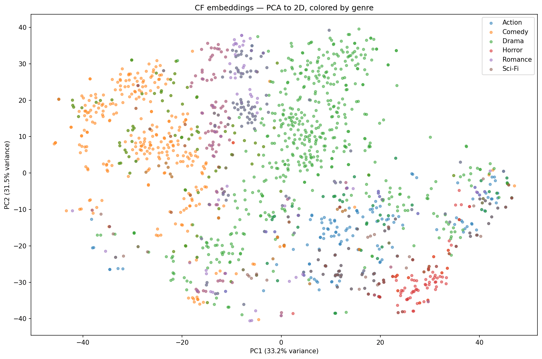
The dense central cluster is popular films — movies that appear in thousands of playlists and co-occur with everything, pulling their embeddings toward the mean. The outliers at the edges are niche films with strong, specific audiences whose vectors got pulled hard in one direction. Crucially: the genre colors are thoroughly mixed throughout. There is no pure-Drama island or pure-Action peninsula. The model did not organize around genre.
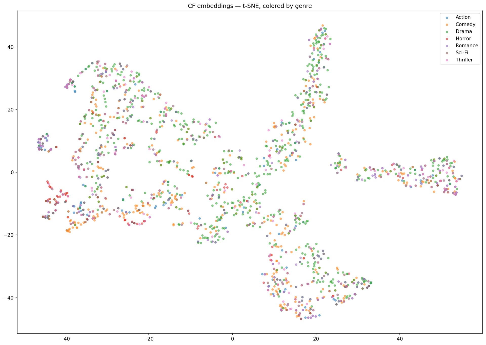
The t-SNE map makes the hidden dimensions legible. Scream and Liar Liar — a horror film and a comedy — land in the same cluster. Contact, In & Out, and Air Force One cluster together despite spanning drama, comedy, and action. The organizing principle is release era and mainstream cultural moment, not genre. The model learned “movies a casual 1997 moviegoer watched in theaters” as a coherent taste dimension without ever being told what year anything came out.
04 Two Spaces, Same Movies
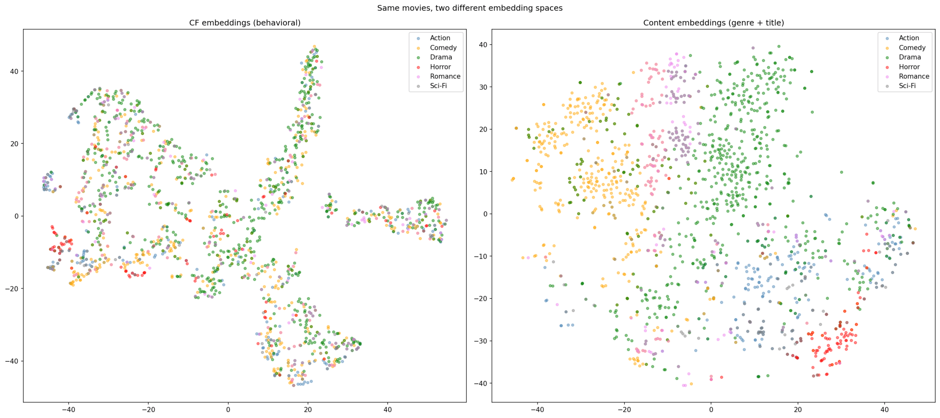
The content plot (right) looks like a well-organized library. Horror clusters in the bottom-right. Romance floats upper-middle. Comedy occupies upper-left. Liar Liar sits deep in the Comedy cluster where you’d expect it. Scream is in the Horror cluster. Everything is where a librarian would put it.
The CF plot (left) looks like a city — messy, overlapping, with neighborhoods that don’t respect administrative boundaries. And that messiness is the point. Look at what it got right that the content plot got wrong: Toy Story, Star Wars, and Return of the Jedi form a tight triangle in the lower-center. In the content plot, these three films are scattered across different regions because their genre flags differ. CF pulled them together because the same people watch all three — families, adventure-lovers, people who build “movie night classics” playlists.
Pulp Fiction is a lone outlier in the far upper-left of the CF map, isolated from the main body. That’s the cinephile signal — the people who rate Pulp Fiction are a specific, self-consistent audience whose co-viewing patterns don’t blend with the mainstream. Content puts Pulp Fiction in a generic central Drama position, indistinguishable from hundreds of other films.
05 The Neighbor Comparison
The most direct way to see the difference: ask each system “what’s most similar to this movie?” and read the results.
| Anchor film | CF neighbors (behavioral) | Content neighbors (genre + title) |
|---|---|---|
| Toy Story Animation · 1995 |
|
|
| Pulp Fiction Crime · 1994 |
|
|
| Star Wars Sci-Fi · 1977 |
|
|
| Scream Horror · 1996 |
|
|
The CF column reads like a playlist someone actually curated. Pulp Fiction’s neighbors are classic films spanning six decades, united not by genre but by the type of person who watches them — the film-literate viewer who works through the canon. Toy Story’s neighbors are critically acclaimed adult dramas, because the users who rated Toy Story are the same people who also sought out prestige films that year. Scream’s neighbors are all 1997 box office releases, because the behavioral signal is “movies that appeared in the same ‘new releases’ playlists.”
The content column reads like a genre search result. Correct, genre-consistent, and largely unhelpful for predicting what any specific person will watch next.
06 Why Content Failed at Cold Start
The counterintuitive result: on sparse movies (≤5 training ratings), content scored 0.000 and CF scored 0.029. The conventional wisdom says content-based approaches should win here precisely because they don’t need behavioral data. What went wrong?
Two things. First, binary genre flags are too coarse. Two movies can both be “Action Thriller 1994” and have nothing in common from a taste perspective. The feature space lacks resolution to discriminate between films that share genre labels but attract entirely different audiences. Richer content features — plot summaries, cast, director, user-generated tags — would close this gap. MovieLens-1M includes user tags, and repeating this experiment there would likely produce the non-monotonic alpha curve the hybrid literature predicts.
Second, cold-start movies in this dataset tend to be niche or unusual films. Their nearest content neighbors by genre and title are other niche films that users also rarely rate — so even when the content similarity is geometrically correct, the recommended films are ones the target user has no history with either. The system correctly finds similar movies; it just finds movies that nobody in the dataset has seen.
07 What This Means for Building Real Systems
No production recommender at scale uses a single approach. The findings here explain exactly why.
CF captures taste identity — the hidden dimensions of human preference that don’t map onto any metadata field. The “cinephile who cross-rates decades” dimension. The “1997 mainstream moviegoer” dimension. The “family adventure night” dimension. These emerge from aggregated human curation and cannot be reverse-engineered from content alone.
Content features handle cold start and long-tail discovery — but only when they’re rich enough. Binary genre flags aren’t. Audio spectrograms, plot embeddings, cast graphs, and user-generated tags are.
The production architecture — Spotify’s three-pronged system, YouTube’s two-tower network, Netflix’s matrix factorization plus graph neural networks — is a direct response to this tradeoff. Start with content for new items. Transition to behavioral embeddings as co-occurrence data accumulates. Blend both in a learned two-tower network that optimizes the mixture end-to-end.
This experiment is a small-scale proof of why that complexity is necessary. Pure CF on 100k ratings already outperforms content by 2× on a coarse evaluation metric. On richer data with richer content features, the hybrid advantage becomes measurable — and at Spotify’s scale of 700 million user-generated playlists, the difference between a 4% and 8% improvement in Recall@20 translates directly to how many users stay on the platform.
08 Resources
Data and tools used in this experiment:
- MovieLens 100K Dataset — GroupLens Research
- Gensim Word2Vec — Radim Řehůřek
- Sentence-BERT (all-mpnet-base-v2) — SBERT.net